Comment faire changer la couleur d’une forme en fonction de la valeur d’une cellule dans Excel ?
Modifier la couleur d’une forme en fonction de la valeur d’une cellule spécifique peut s’avérer une tâche particulièrement utile dans Excel. Par exemple, si la valeur de la cellule A1 est inférieure à 100, la forme devient rouge ; si elle se situe entre 100 et 200, elle passe au jaune ; et dès qu’elle dépasse 200, elle vire au vert, comme le montre la capture d’écran ci-dessous. Cet article vous explique comment adapter automatiquement la couleur d’une forme selon la valeur d’une cellule.

Modifier la couleur d’une forme en fonction de la valeur d’une cellule à l’aide d’un code VBA
Modifier la couleur d’une forme en fonction de la valeur d’une cellule à l’aide d’un code VBA
Le code VBA ci-dessous vous permet d’ajuster automatiquement la couleur d’une forme en fonction de la valeur d’une cellule. Suivez ces étapes :
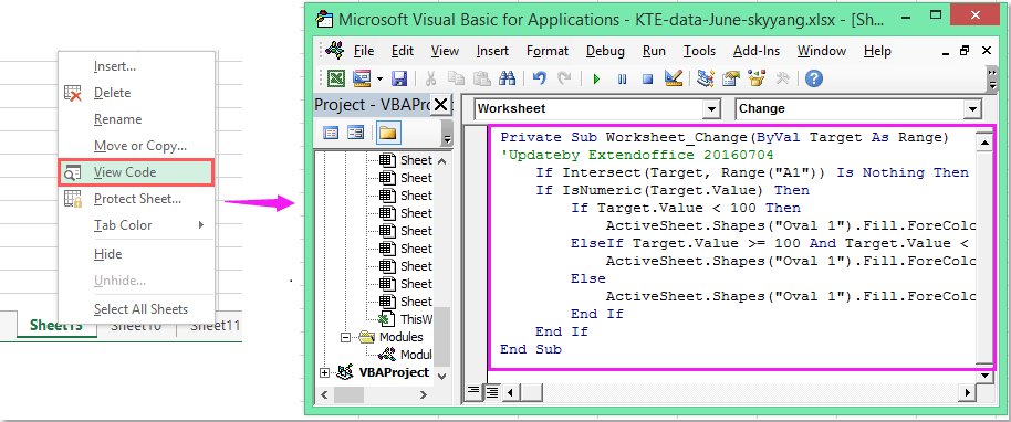
1. Cliquez avec le bouton droit sur l’onglet de la feuille dans laquelle vous souhaitez modifier la couleur de la forme, puis sélectionnez Afficher le code dans le menu contextuel. Dans la fenêtre Microsoft Visual Basic pour Applications qui s’ouvre, copiez et collez le code suivant dans la fenêtre vierge du Module.
Code VBA : Modifier la couleur d’une forme en fonction de la valeur d’une cellule :
Private Sub Worksheet_Change(ByVal Target As Range)
'Updateby Extendoffice 20160704
    If Intersect(Target, Range("A1")) Is Nothing Then Exit Sub
    If IsNumeric(Target.Value) Then
        If Target.Value < 100 Then
            ActiveSheet.Shapes("Oval 1").Fill.ForeColor.RGB = vbRed
        ElseIf Target.Value >= 100 And Target.Value < 200 Then
            ActiveSheet.Shapes("Oval 1").Fill.ForeColor.RGB = vbYellow
        Else
            ActiveSheet.Shapes("Oval 1").Fill.ForeColor.RGB = vbGreen
        End If
    End If
End Sub
2. Dès que vous saisissez une valeur dans la cellule A1, la couleur de la forme change automatiquement en fonction de la valeur définie.
Remarque : Dans le code ci-dessus, A1 correspond à la cellule dont la valeur détermine le changement de couleur de la forme, et Oval 1 est le nom de la forme insérée. Vous pouvez les adapter selon vos besoins.
Meilleurs outils de productivité Office
Boostez vos compétences Excel avec Kutools pour Excel et découvrez une efficacité inégalée.Kutools pour Excel propose plus de 300 fonctionnalités avancées pour améliorer votre productivité et Gagner du temps.Cliquez ici pour obtenir la fonctionnalité dont vous avez le plus besoin...
Office Tab apporte une interface à onglets à Office et rend votre travail bien plus facile
- Activez l’édition et la lecture par onglets dans Word, Excel, PowerPoint, Publisher, Access, Visio et Project.
- Ouvrez et créez plusieurs documents dans de nouveaux onglets de la même fenêtre, plutôt que dans de nouvelles fenêtres.
- Augmente votre productivité de 50 % et vous fait économiser des centaines de clics de souris chaque jour !
Tous les compléments Kutools. Un seul installateur
Kutools for Office regroupe les compléments pour Excel, Word, Outlook et PowerPoint, ainsi que Office Tab Pro, ce qui en fait le choix idéal pour les équipes travaillant à travers les applications Office.
- Suite tout-en-un— Compléments Excel, Word, Outlook et PowerPoint + Office Tab Pro
- Un seul installateur, une seule licence— installation en quelques minutes (compatible MSI)
- Fonctionne mieux ensemble— productivité optimisée dans toutes les applications Office
- Essai gratuit de 30 jours avec toutes les fonctionnalités— aucune inscription, aucune carte bancaire
- Meilleur rapport qualité-prix— économisez par rapport à l’achat de compléments individuels